A bike camera, on its own, can now measure the gap an overtaking car leaves: typically within 18 cm of a hardware sensor, tested on 3,961 real passes from 284 riders it had never seen. This page shows exactly how, on real footage, step by step.
real PassBox footage · overlays computed by the method
Every clip here is from a rider the model never trained on. The sensor number is the answer key; the model never sees it. The whole page uses the same colours: blue for the sensor and the tyre-contact point, amber for the model's estimate, magenta for road geometry, white for the car detector.
Chapter 1
Why this matters
Australian road rules require a driver to leave at least 1 metre when overtaking a cyclist, or 1.5 metres where the speed limit is above 60 km/h. The rule is rarely enforced because a close pass is over in two seconds and nobody can measure it afterwards.
The PassBox project proved it can be measured. Riders carried a box with an ultrasonic distance sensor and two Garmin cameras. Over several years it recorded 104,596 overtaking events, each with a six-second video clip and the sensor's reading of the true gap, accurate to about 2 cm.
Sensors are rare. Cameras are everywhere: many cyclists already ride with one. If the gap could be read from the video alone, with an honest statement of how far off it might be, every bike camera becomes a measuring instrument, and the PassBox archive becomes the answer key to test it against.
That is what this project set out to do, and what the rest of this page explains: how the computer reads distance out of pixels, how close it gets, where it fails, and how to put it to work.
Chapter 2
What the camera sees
The footage is harder than it looks. A camera on the back of a bike shakes, leans into corners, faces the sun, and films in rain and at night. The archive also arrived in a reduced form: every clip was shrunk to 640 pixels wide, cropped by an unrecorded amount, and re-compressed. The settings that normally anchor a measurement, such as the camera's focal length and where the middle of the lens is, were lost.
A clip exactly as delivered.
Three quirks worth knowing
Pixels are not distances. A car 1 metre away and a car 2 metres away are the same colour, the same shape, and just different sizes. Everything below is about recovering real-world scale from image content.
The camera is a mystery. Because of the crop, the lens looks about twice as zoomed-in as the camera's specification says. A calibration network later confirmed this, and correcting it helped every measurement.
Two cameras in one picture. Many clips stack the front and rear camera on top of each other, with the seam not quite in the middle. The pipeline has to find the seam and work on one pane.
One pane of a stacked clip at the moment of closest approach. The method works on this pane only.
Chapter 3
How the computer measures
The method is a chain of six steps. Each step uses a different piece of software, and each one is shown here on real footage. The thing that makes the whole chain work is a single idea from perspective: where a tyre touches the road, the maths gets simple.
Step 1. Find the car
A general-purpose object detector called YOLOX looks at every frame and draws a box around anything that is a vehicle. A tracker then follows the one car that comes closest, frame to frame, and drops the track when it drifts onto a parked or oncoming car, which happens in almost every clip after the pass.
The detector was not trained by this project. It is an open-source model that already knows what cars look like.
Step 2. Find where the tyre meets the road
This is the model this project built. It takes the car's box and marks eight points: the hub of each wheel (amber) and the exact pixel where each tyre touches the road (blue). From a rear camera only the near rear tyre is reliably visible, so that single contact point carries the measurement.
The first version learned only from a driving simulator and found the tyre in 21% of real frames. Two rounds of teaching it on its own confident real-footage detections raised that to 64% and then 85%. Chapter 7 tells that story.
Step 3. Find the horizon
To turn a contact point into a distance you need to know where the horizon sits in the image and how the camera is turned. Neither is recorded. But lane lines and kerb edges all point to the same vanishing point on the horizon. The software finds straight oblique edges (magenta), votes on where they meet, and keeps the most agreed-on answer across the whole clip.
Finding the horizon per clip, rather than assuming one, was the single biggest improvement in the first phase of the work. It also reveals the camera's sideways turn, which was off-centre by a median of 245 pixels.
Step 4. Find the shadow under the car
The road under a car is in shadow. The bottom edge of that dark strip is another reading of where the car meets the ground, and it is measured across dozens of columns of pixels rather than at one point, so it is steadier in bad light. It came from a research review in the middle of the project and is a weak cue on its own, but it adds a little in the final combination.
Step 5. Turn pixels into centimetres
The geometry cue live. The amber bar is one frame's sideways offset; the running number is the median so far.
For a point on the road, the number of pixels it sits below the horizon tells you how far away it is along the road, and how far it sits left or right of the camera's centre line tells you the sideways gap. The camera's height does the scaling: about 48 cm for a rear-rack mount, a value the data itself confirmed. The focal length, the mystery number, cancels out of the calculation entirely. That is why the contact point matters so much: it is the one place where the unknown camera does not get in the way.
One frame is not enough. Each contact point is a noisy reading, so the method takes the median over the whole pass, typically about 50 usable frames, and that is the geometry cue.
Step 6. Ask a depth network for a second opinion
The frame at closest approach.The same frame as seen by Depth-Anything-V2, a network that guesses distance from texture and shading. Pale is near, dark is far.
A modern depth-estimation network can look at a single photograph and guess how many metres away each pixel is. On this cropped, re-compressed footage its guesses are rough, often several metres out, but they are independent of the geometry, so they are sampled at the tyre-contact point and handed to the final combination as one more clue.
Chapter 4
Combining the clues
No single cue is good enough. The geometry, the shadow line, a wheel-as-ruler estimate and the depth network each land around 26 to 30 cm of typical error on their own, about the same as simply guessing the average pass every time. The gain comes from combining them.
A small statistical model (gradient-boosted decision trees, about 300 of them) takes roughly twenty numbers per pass: the four cues, how confident each one is, how large the car grew in the frame, how low its box sat, the vehicle type, and the recovered camera settings. It learns from passes with a sensor reading how to weigh them, and then produces one number per pass.
Scrambling each clue in turn and watching the error rise shows what the model actually leans on:
What the final model relies on
Twelve most important inputs. Measured on the full 3,961-pass set.
The honest reading is that the car's apparent size is the strongest single clue, as a peer paper on the same problem also found. The tyre-contact point is still the backbone: it anchors the geometry cue, the wheel-ruler cue and where the depth network is sampled, and the horizon it needs is what makes the model work on a new camera at all. The combination is what reaches 18 cm.
Why a decision-tree model and not a bigger neural network? With a few thousand labelled passes, a small model that combines physically meaningful measurements beats a large network that has to discover them. A full video network trained on all 104,000 clips is the next step, not the current one.
Chapter 5
How well it works
18.0cm typical error
Mean absolute error against the ultrasonic sensor, on 3,961 passes under 2 metres, from 284 riders excluded from training.
14.4 cm
median error: half of all passes are closer than this
38.0 cm
90th percentile: nine in ten passes are within this
26.7 cm
error if you guessed the typical pass every time
98%
of confident "under 150 cm" calls were correct (286 of 292)
How the scoring was done
The model is scored only on riders it never trained on. The passes were split into five groups by rider, the model was trained on four and tested on the fifth, and this was repeated so every pass was tested exactly once by a model that had never seen that rider, bike, camera mount or route. Scoring on entirely unseen rides instead gives 18.1 cm, so the result is not memorisation.
Once a rider has a few sensor-labelled passes, the model can learn that rider's camera offset. That calibration takes the error from 18.5 to 18.0 cm. Without it, the uncalibrated figure is 18.5 cm.
Video estimate against the sensor, one dot per pass
3,961 passes. A dot on the diagonal is a perfect match. Hover a dot to read it.
How far off each pass was
Difference between video and sensor, in 5 cm bins.
The same numbers as a table
Measure
Value
Passes scored
3,961
Riders, none seen in training
284
Mean error, unseen riders
18.5 cm
Mean error, unseen rides
18.1 cm
Mean error, with per-rider calibration
18.0 cm
Median error
14.4 cm
90th percentile error
38.0 cm
Rank correlation with the sensor
0.68
"Under 150 cm" calls at 95% confidence
292, 286 correct
The legal output
For evidence, an average error matters less than a defensible claim. The system makes the one-sided statement "this pass was under 150 cm" only when a calibration step, run on a separate set of riders, supports 95% confidence. On the test set it made 292 such claims and 286 were right. Forensic measurement standards ask for exactly this form: a claim with a known error rate, and silence when the quality checks fail.
Context: the only comparable study
One published paper reports 13 to 14 cm on this exact task. It used one calibrated bike, 96 passes and video at three times this resolution. PassBox's own learned model, trained on the full archive, reports 29 cm. At multi-rider scale on degraded footage, 18 cm is the strongest known result.
Chapter 6
Where it struggles
Error by how close the pass really was
The closest passes, which matter most, are the hardest.
Very close passes read too wide. Under 80 cm the car fills the frame, the tyre is often cut off at the bottom edge, and the model drifts toward the typical pass. Several of the close passes in the stage above show this: a 64 cm pass reads as 90 or 100. For a safety tool that is the wrong direction to err, so the confidence calibration abstains in these cases rather than making a claim.
The answer key has its own definition. The ultrasonic sensor measures whatever is nearest, usually a wing mirror or body panel, at its own moment of closest approach. The camera measures the tyre during the approach. That gap alone is 6 to 10 cm, so no video method can score much below 13 to 17 cm against these labels. The remaining room for improvement is real but bounded.
Dusk, and the hard cases generally. The tyre model finds the contact point in 85% of frames in daylight, 65% at night, and 71% at dusk after the second round of training, up from 4% at dusk for the first version. When the horizon cannot be found (about 30% of clips) the model falls back to a per-camera average and becomes less confident.
More data stopped helping. Going from 350 to 1,550 passes removed 2.9 cm of error. Going from 1,550 to 3,961 removed 0.3 cm. The next gains have to come from better methods or better source footage, not more clips.
Chapter 7
How we got here
The work ran from June to November 2026 in about 600 commits, almost all of it on a laptop. Four phases.
Phase A. Does the geometry work on real footage at all?
232 real clips, a tyre model that had only ever seen a driving simulator, and the perspective maths. Every number was checked against the simplest possible rival: guessing the median pass. The first attempt, measuring from a single frame, lost to that rival. Pooling frames over the whole pass helped. Finding the horizon per clip from lane lines made the geometry physically honest for the first time: the fitted camera height came out at 35 to 48 cm, a real rack-mount height rather than a number the fit had invented. Result: 28.8 cm on passes under 2 metres, level with PassBox's own model.
Phase B. Teach the tyre model on real roads
The simulator-trained model placed the point correctly when it fired, but it rarely fired on real frames, and least of all at night, in rain and when the car was close. The fix was self-training: harvest its own most confident, geometry-verified detections on real frames as labels, and fine-tune on those with heavy darkening and blur. Two rounds of that produced versions 2 and 3.
How often the tyre model finds the contact point
Share of tracked frames with a confident contact point, by weather, on 43 held-out riders. Versions 2 and 3 compared at a matched confidence threshold.
Dusk and fog have few frames (48 and 28), so those bars have wide uncertainty. Version 3 trades a little rain and overcast performance for large gains in the dark.
Phase C. Ask what else is possible
With the error stuck around 26 cm, the project paused to consult: an audit by an external AI model, plus a reading of about 150 papers across computer vision, forensic video analysis and even sonar tracking. The verdict was that 26 cm was bias, not a physical floor, and the plan it produced is what Chapters 3 and 4 describe: car-size features, the shadow line, the wheel-as-ruler, a depth network, recovering the camera settings, strict rider-grouped scoring, and the calibrated legal claim.
Phase D. Execute and scale
Error as the method and the test set grew
Mean absolute error in cm. The plateau near 18 is the current state.
What was tried and closed
Single-frame measurement. No usable signal. Only whole-pass aggregation works.
Anything needing two wheels (wheelbase as a ruler, full pose). The rear camera reliably sees only the near rear wheel.
Number plates as rulers. 8 to 25 pixels wide in this footage. Too small.
Video super-resolution. Sharpens by moving edges, which corrupts measurement.
Audio. Compressed mono audio cannot tell 1 m from 2.5 m.
Per-frame lean correction, box-corner shortcuts, extrapolating to the exact pass moment. All null or harmful.
Cloud simulator rendering. Graphics driver failures on every host tried. Self-training on real footage replaced it and cost about $1 of cloud time in total.
The Phase B demo reel: what version 2 trained on, then version 2 running on never-seen clips across clear, overcast, dusk, fog, rain and night with the sensor value on screen. Note that this reel uses the older Phase A calibration, so its close passes show the "about a metre" floor that Phases C and D later attacked.
Chapter 8
Other cameras and fisheye
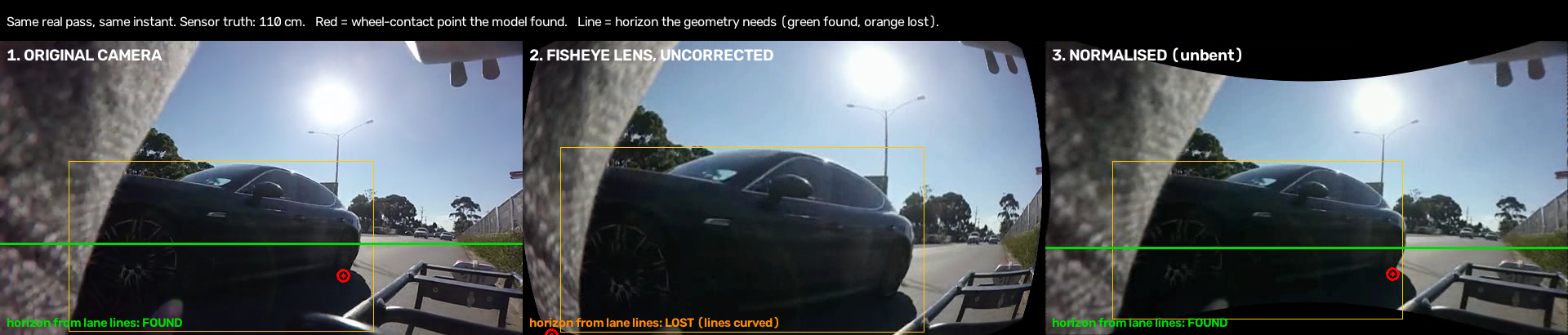
Every camera bends the world differently. A wide-angle action camera bows straight lines outward; a narrow lens barely bends them. The method was built on one camera's view, so a different lens moves where tyres and road edges land in the frame. The plan for new cameras has two parts: calibrate each camera once by filming a checkerboard, then straighten every frame to a standard view before the method runs. One method, every camera.
One pass (sensor 110 cm) at the same instant through three conditions. Left: original, horizon found, contact on the tyre. Middle: the frame bent through a real fisheye lens profile; the horizon finder gives up and the contact point slides. Right: straightened with the lens profile; both recover.
Condition on 384 clips
Mean error
Median
Clips with a confident horizon
Original footage, re-encoded once (control)
20.3 cm
17.2 cm
70%
Fisheye lens, uncorrected
22.4 cm
18.4 cm
38%
Fisheye lens, straightened
21.3 cm
17.6 cm
69%
An uncorrected fisheye camera costs about 2 cm of mean error and halves the clips where the horizon can be found. Straightening recovers the median completely and most of the mean. The experiment also found that a single extra round of video compression costs about 2.5 cm of median error on its own, so a product must straighten frames in memory, never by writing an intermediate video.
The tools exist on the branch: a checkerboard calibrator, a frame normaliser that handles both fisheye and simple lens models, and a synthetic test that proves them without a camera. The next real camera to be calibrated is the one Scott bought; the instructions are in realworld/fisheye/FISHEYE-PLAN.md.
Chapter 9
The models and weights
Four trained models take part. One was built here; the others are open models used as published. Everything built here is downloadable from this page.
The tyre-contact model (built in this project)
A small keypoint network: a MobileNetV3-small backbone with a deconvolution head. It takes a 512 × 512 crop around the car and outputs eight 128 × 128 heat maps, one per keypoint (hub and contact for each of four wheels). The peak of each map, refined to sub-pixel precision, is the keypoint. About 21 MB, and fast enough to run on a phone or in a browser through ONNX Runtime.
Version
Trained on
Use
Files
v3
v2 plus 8,179 more self-labelled real frames, night-heavy (9,979 total)
Default for the distance pipeline and for hard conditions
Each ONNX file is 21.6 to 21.9 MB. Checksums (SHA-256, first 16 characters): v3 onnx 1285d992f21bbee8, v3 pt 498768fd23d5d6d8, v2 onnx 69348ebc7b1dab27, v2 pt 454a2687e35174b2, v1 onnx 24800ee9fbe1e7a7, v0 onnx 504ce4f201556d0f. Input: image[1,3,512,512], normalised with ImageNet mean and standard deviation. Output: heatmaps[1,8,128,128]. Keypoint order: FL_hub, FL_contact, FR_hub, FR_contact, RL_hub, RL_contact, RR_hub, RR_contact. Versions 2 and 3 produce much higher confidence scores than version 1, so any threshold must be re-tuned from the metrics file rather than carried over.
A caveat on how the tyre model was trained. Versions 2 and 3 learned from the previous version's own confident predictions on real frames, not from human-drawn labels. Spot checks of its new detections were 13 of 14 correct, and the sensor-based distance results are the external test. But there is no independent human labelling of real frames yet; that would be a worthwhile addition.
The combination model
A scikit-learn HistGradientBoostingRegressor (300 trees, depth 4) over the per-pass features, with a companion 90th-percentile model for the confidence interval. It is retrained in under a minute from the committed feature journals by realworld/accuracy/consult_fit.py; a trained copy and its feature list are here: fusion_hgb.joblib · feature list. The per-pass features themselves (4,993 clips, every frame's box, keypoints, shadow line, horizon and depth) are the rich3_*.jsonl journals in realworld/accuracy/.
Open models used as published
Car detector: YOLOX-S, Megvii, Apache-2.0. yolox_s.onnx (36 MB).
Camera recovery: AnyCalib, used once per clip to recover the focal length and image centre from the crop.
Reproducing everything
All code, journals and reports are in the realworld/ folder of the obc-wheel-trainer repository on branch claude/wheel-detection-model-1d3785. Start with realworld/accuracy/FINAL-REPORT.md. The four-stage pipeline (run_cohort3.sh) resumes from its journals and survived several laptop restarts without losing work. The media on this page was rendered by realworld/site/build/render_clip_media.py, which runs the real pipeline on each clip.
Chapter 10
Putting it to work
The method is a batch process: a six-second clip goes in, a distance with a confidence range comes out. Measured on a laptop, one pass takes about 15 seconds of processing at full frame rate and about 5 seconds at the 10 frames per second the pipeline normally uses. That makes the system cheap to run and simple to host. Here is a drafted architecture and a plan.
What already exists
Steps 3 and 5 are code today. The trigger (detector plus tracker, release-grade) lives in Scott's openbikecam repository. The measurement chain is the four-stage pipeline on this branch, with the lens normaliser ready for the first calibrated camera. The combination model retrains in under a minute.
What to build
A thin upload path, a queue, the worker container, a results schema, and the two outputs people actually want: a rider's own dashboard, and an evidence pack for a single pass. None of it is research.
Cost sketch
At 5 seconds per pass per CPU core, a 4-core server processes about 70,000 passes a day. That is a €20 to €40 per month machine, or a container platform billed per second. Storage is about 1 MB per clip plus the overlay video; 100,000 passes is roughly 300 GB, under $5 a month on R2. GPU time is only needed for retraining: about $0.34 an hour on a rented RTX 4090, and a full retrain of the tyre model is a few hours.
Running on the device instead
Both the detector and the tyre model are ONNX files that run in a browser or a phone app. A fully on-device version is feasible for riders who do not want to upload footage; the depth network is the only heavy part and it is optional.
A plan in four stages
Stage
What happens
Done when
1. Prove it on a new camera weeks 1 to 4
Film the checkerboard on Scott's camera, fit its lens profile, straighten a few of his rides, run the batch pipeline and compare against anything with a known distance. Fix whatever the new lens breaks.
The method runs end to end on a camera it has never seen and the plumb-line and horizon checks pass.
2. Hosted batch service months 2 to 3
Package the worker as a container, add the queue and results store, and a simple upload page. Process rides overnight and email a report.
Ten riders upload rides and get per-pass distances with confidence bounds without anyone touching a terminal.
3. Evidence and dashboards months 3 to 5
Evidence export per pass (clip, overlays, method statement, known error rate), rider dashboard, aggregate maps for councils. Decide and document the abstention rules.
A report has been reviewed by someone who handles road-safety complaints and they can follow it without help.
4. Improve the measurement in parallel
Ask the PassBox team for original-resolution footage and the sensor's full time series per pass. Train the end-to-end video model on all 104,000 clips. Add timestamp-aware trajectory fitting and a newer video-depth model. Human-label a few hundred real frames to audit the tyre model.
Error moves measurably toward the 13 to 17 cm floor, and night and occluded passes stop being the weak spot.
Two rules for any deployment. Report the calibrated range, not a bare number, and stay silent when the quality checks fail. And wherever a real sensor exists, keep it primary; the camera is for everyone who does not have one.
Chapter 11
Glossary and questions
Close pass
A driver overtaking a cyclist with less than the legal minimum gap: 1 m at 60 km/h and below, 1.5 m above that, in most Australian states.
Ultrasonic sensor
A device that times an echo to measure distance, like a bat. PassBox used one to record the true gap for every pass. It is the answer key throughout.
Mean absolute error
Take every pass, measure how far the video estimate is from the sensor, ignore the sign, and average. 18 cm means the typical pass is off by about that much.
Median error
The middle value when the errors are sorted. Half the passes are closer than it. Less affected by a few bad cases than the mean.
Keypoint
A specific named point in an image that a model learns to locate, such as "where the rear-left tyre touches the road".
Horizon and vanishing point
Parallel lines in the world, such as lane edges, meet at a vanishing point in a photograph. All such points for level ground sit on one line, the horizon. Its position in the image depends on how the camera is tilted.
Focal length
How zoomed-in a camera is. Unknown for these clips, which is why the method is built around the contact point, where it cancels out.
Held-out riders
Riders deliberately kept out of training so the model is scored on people, bikes and camera mounts it has never seen.
Calibrated claim
A statement with a known error rate, such as "under 150 cm, right 95% of the time", produced only when the evidence supports it.
Self-training
Using a model's own most confident predictions as labels to train its next version, with checks to avoid teaching it its own mistakes.
ONNX
A file format for trained models that many programs can run, including browsers and phones.
Questions people ask
Could this be used to fine a driver?
Not on its own. It produces a distance with a known error rate, and an evidence pack that shows how the number was obtained. Whether that meets a legal standard is for the people who set such standards. The design follows forensic measurement practice: a one-sided claim, a stated confidence, and abstention when quality checks fail.
Why not just use the sensor?
Where a sensor exists, use it; it is more accurate. The point of the camera method is the far larger number of riders who have a camera and no sensor, and the fact that the video is itself the evidence.
Does it work at night?
Partly. The tyre model now finds the contact point in about two thirds of night frames, up from 6% for the first version. The distance result at night has not been scored separately at scale, and the plan treats night and dusk as low-confidence until it has.
Does it work with my camera?
It will, after a one-time calibration: film a printed checkerboard for a minute, and the software fits your lens. Until a camera has been calibrated, treat its numbers as rough. The archive camera was a Garmin VIRB X; the experiment in Chapter 8 shows what an uncorrected wide lens costs.
Why does the model need the car's size if the geometry is so clever?
Because the geometry is only as good as its inputs, and on this footage every input is noisy. A big car close to the camera is a strong, simple signal, and the combination model uses whatever reduces error on the sensor-labelled passes. The geometry is what lets the method transfer to a new camera; the size cue is what sharpens it on this one.
How was the error measured so it cannot be fooled?
Every reported number is on riders the model never saw, in a five-way rotation so each pass is tested by a model that excluded its rider. Earlier, easier scoring on random splits gave 26 cm; the strict scoring changed the answer by under 1 cm, which is itself evidence the result is real.